Next: Array Organisation in FASTEST Up: Detailed Code Description Previous: General Structure of the Contents Index
In the modelling of a flow problem, each CV provides one algebraic equation. Volume integrals are calculated in the same way for every CV, but the CVs on the domain boundaries require special treatment. The fluxes on the boundaries must either be known, or be expressed as a combination of interior values and boundary data. Generally, either the value of the variable at the boundary (Dirichlet boundary conditions) or its gradient in a particular direction (Neumann boundary condition) or a combination of both is given. If the value of the variable is given, there is no need to solve for it and the known values are used in the equations. If the gradient at the boundary is given, a suitable approximation can be used to calculate the boundary value of the variable. The approximation must be based on one-sided differences or extrapolations since there are no nodes outside the boundary.
In FASTEST3D the following boundary condition types are implemented:
The values in parentheses denote the value of the boundary condition used in the code of FASTEST3D.
FASTEST3D gets the information of boundary types for each domain from the boundary condition input data for the grid file. In the boundary conditions file, after the connecting faces of the blocks are defined, the boundary faces are introduced for each block. Here, ``SOL'', ``MIR'', ``OUT'', ``INL'' and ``PER'' stand for wall, symmetry, outlet, inlet and periodic boundary conditions respectively.
Inlets are generally Dirichlet boundary conditions. This means that the velocity components at the inlet are known and are assigned to the boundary nodes. The boundary fluxes are then calculated from their discretized expressions.
In case the boundary fluxes are known, they are simply used in flux balance equations and the boundary values are then evaluated from the discretized flux expressions.
Usually, all quantities at the inlet boundary are prescribed. If the conditions at the inlet are not well known, it is useful to move the boundary as far from the region of interest as possible. All convective fluxes can be colculated since the velocity and the other variables are known. The unknown diffusive fluxes can be approximated using known boundary variables and one-sided finite difference approximations for the gradients.
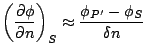
Prescribed gradient (usually zero) of all quantities are used on an outflow surface. Outlet boundaries should be as far of the main region of interest as possible, since there is usually little information about the flow here. When it is far enough away from the region of interest, the assumption of a zero gradient along grid lines is sufficient for high Reynolds number flows. This means that for the flux, a first order upwind approximation is used.
In FASTEST, the zero gradient condition is implicitly implemented. For example,
at the east face, the first order backward approximation gives
![]() .
When this expression is used in the discretized equation for the CV next to the
boundary, equation becomes:
.
When this expression is used in the discretized equation for the CV next to the
boundary, equation becomes:
![]()
So the boundary value ![]() does not appear in the equation.
does not appear in the equation.
If higher accuracy is required, higher-order and one-sided finite difference approximations of the derivatives must be used. Both convective and diffusive fluxes have to be expressed in terms of inner nodes variable values.
On the walls, no-slip boundary condition (viscous fluid sticks to
solid boundary, fluid velocity is equal to the wall velocity)
exists. Since there is no flow through the wall, convective fluxes
of all quantities are zero. For scalar quantities like thermal
energy, they may be zero (adiabatic walls), they may be specified
(prescribed heat flux), or the value of the scalar may be prescribed
(isothermal walls). If the flux is known, it can be inserted into
the conservation equation for the near wall CVs. If the value of
![]() is specified at wall, it is possible to approximate the
normal gradient of
is specified at wall, it is possible to approximate the
normal gradient of ![]() using one-sided differences. With the same
approximation
using one-sided differences. With the same
approximation ![]() value at the wall can also be described when
the flux is described.
value at the wall can also be described when
the flux is described.
 |
(2.1) |
FIGURE (Not added in cvs)
Here, P' is located on the normal n, ![]() is the distance
between the points P' and S, see FIGURE.
is the distance
between the points P' and S, see FIGURE.
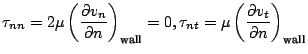
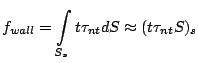
The viscous stresses at the wall can be described as:
 |
(2.2) |
As it is seen, normal viscous stress is zero at the wall. This can be
found out following from the continuity equation. The discrete version
of the shear force per unit area at the wall (![]() ) is:
) is:
 |
(2.3) |
where
![]() is the difference between the velocities parallel
to the wall at the near wall node P and the wall node (S in FIGURE).
In case of a laminar flow, velocity gradient at the wall may be
calculated by assuming a linear distribution from the wall to the
first near-wall node. However in turbulent flows, this would be true
only for the very thin viscous sublayer near the wall, and generally,
the first computational node lies within the turbulent region. To
bridge the near-wall region, wall functions are used in
k-
is the difference between the velocities parallel
to the wall at the near wall node P and the wall node (S in FIGURE).
In case of a laminar flow, velocity gradient at the wall may be
calculated by assuming a linear distribution from the wall to the
first near-wall node. However in turbulent flows, this would be true
only for the very thin viscous sublayer near the wall, and generally,
the first computational node lies within the turbulent region. To
bridge the near-wall region, wall functions are used in
k-
![]() turbulent model.
turbulent model. ![]() is equal to
is equal to ![]() for
laminar flows, while it is formulated as follows for turbulent flows.
for
laminar flows, while it is formulated as follows for turbulent flows.
 |
(2.4) |
Here ![]() is the dimensionless distance of P' to the wall, and it is defined as:
is the dimensionless distance of P' to the wall, and it is defined as:
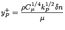 |
(2.5) |
For the validity of the k-
![]() model,
model, ![]() should be
greater then 30, however in FASTEST, for practical reasons, this value
is taken as 11.63. For the values bigger than 11.63 are considered
turbulent while for the smaller values laminar functions are applied.
should be
greater then 30, however in FASTEST, for practical reasons, this value
is taken as 11.63. For the values bigger than 11.63 are considered
turbulent while for the smaller values laminar functions are applied.
After the shear stress ![]() is calculated, shear force at the
wall can be expressed as:
is calculated, shear force at the
wall can be expressed as:
 |
(2.6) |
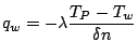
In temperature dependent flow cases, two kinds of wall boundary conditions exist:
In case of adiabatic wall, the flux is set to zero and the wall temperature is calculated by extrapolation. Prescribed wall temperature case requires the distinction between the turbulent and laminar flows. The specific heat flux on wall can be expressed as:
 |
(2.7) |
Here, ![]() and
and ![]() are temperature at the cell center P and on the
wall respectively.
are temperature at the cell center P and on the
wall respectively. ![]() is defined as
is defined as
![]() for
laminar flows (
for
laminar flows (![]() stands for Prandtl number). For turbulent
case
stands for Prandtl number). For turbulent
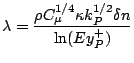
case ![]() is:
is:
![$\displaystyle \lambda = \frac {\rho C^{1/4}_{\mu} \kappa k^{1/2}_P \delta n } {\sigma^t_T \left[ \ln(Ey^+_P)+ P_f \kappa \right]}$](img37.png) |
(2.8) |
![]() is the emprical constant called turbulent Prandtl number.
is the emprical constant called turbulent Prandtl number. ![]() is a
function defined in terms of
is a
function defined in terms of ![]() and
and
![]() . The heat flux through a
wall cell face can be evaluated by:
. The heat flux through a
wall cell face can be evaluated by:
 |
(2.9) |
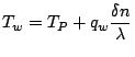
The same expression can be used to calculate the wall temperature when the heat flux is prescribed:
 |
(2.10) |
In many flows, there are one or more symmetry planes. At a symmetry plane, the convective fluxes of all quantities are zero. Besides, the gradients normal to the boundary for all scalar quantities and the velocity component parallel to the symmetry plane are zero.
 |
(2.11) |
where ![]() represents all scalar variables and the parallel velocity component.
represents all scalar variables and the parallel velocity component.
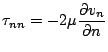
Shear force (![]() ) at the symmetry plane is zero, however, there is a
normal stress acting at such a boundary:
) at the symmetry plane is zero, however, there is a
normal stress acting at such a boundary:
 |
(2.12) |
The resulting force on the symmetry plane can be found having the surface
integral of ![]() as follows:
as follows:
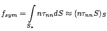 |
(2.13) |
The derivative (
![]() ) can be discretized as:
) can be discretized as:
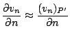 |
(2.14) |
since the normal component at S is by definition equal to zero. The
interpolation factor ![]() which will be used to define variable value at
P' can be found as (Note that according to the FIGURE, P' lies between P and
W. Therefore, here W node is used to find the interpolation function):
which will be used to define variable value at
P' can be found as (Note that according to the FIGURE, P' lies between P and
W. Therefore, here W node is used to find the interpolation function):
 |
(2.15) |
where ![]() ,
, ![]() and
and ![]() are the unit vector representation of
are the unit vector representation of
![]() in global cartesian coordinate:
in global cartesian coordinate:
| (2.16) |
If the open form (in terms of coordinates, angles and interpolation factors)
of the discretized equation for ![]() is used in force equation defined above,
is used in force equation defined above,
![]() -,
-, ![]() - and
- and ![]() -component of the force give contributions for the central
coefficient
-component of the force give contributions for the central
coefficient ![]() and the source term S of u-, v- and w-momentum equations
respectively.
and the source term S of u-, v- and w-momentum equations
respectively.
Usually, the mass flow rate at the inlet is specified and extrapolation is used for the outlet mass flow rate. However, in some cases the mass flow rate is not known, but the pressures at the inlet and the outlet are prescribed. In this kinds of flows, velocity cannot be prescribed. It has to be extrapolated from the interior flow. The pressure gradient at the boundary can be approximated using one-sided differences.
The boundary velocities need to be corrected to satisfy the mass conservation
(the mass flux corrections (![]() ) are not zero at the boundaries where the
pressure is specified). On the other hand, the boundary pressure does not need
to be corrected (
) are not zero at the boundaries where the
pressure is specified). On the other hand, the boundary pressure does not need
to be corrected (![]() ).
).
This boundary type is a special case of the the wall boundary. It is used for defining coupling faces in fluid-structure interaction problems. Other than that it is treated the same way as walls; the no-slip condition applies.